[16주차 - Day2] Basic Recommendation System 구현 I

ML 기반 추천 엔진 : 컨텐츠 기반 추천 엔진 개발

1. 인기도 기반 추천 개발

Cold Start 이슈가 존재하지 않음

인기도의 기준을 어떻게 설정할 지 고민     ex)평점, 매출, 최다 판매 등

사용자 정보에 따라 확장 가능

개인화되어있지 않음

아이템의 분류 체계 정보 존재 여부에 따라 쉽게 확장 가능

인기도를 다른 기준으로 바꿔 다양한 추천 유닛 생성 가능

+기타 Cold Start 이슈가 없는 추천 유닛

현재 사용자들이 구매한 아이템

현재 사용자들이 보고 있는 아이템(영화, 강좌 등)

 

실습

영화 추천 데이터(TMDB 데이터셋 사용)를 가지고 인기도 기반 추천 엔진 개발

인기도는 전체 인기도, 장르 내 인기도(일종의 분류 체계) 카테고리를 지원

데이터셋 : https://www.kaggle.com/tmdb/tmdb-movie-metadata

TMDB 5000 Movie Dataset

영화 정보는 tmdb_5000_movies.csv, 연출/배우에 대한 정보는 tmdb_5000_credits.csv

1. 입력데이터 로딩

import pandas as pd
import numpy as np

movies = pd.read_csv("https://grepp-reco-test.s3.ap-northeast-2.amazonaws.com/tmdb_5000_movies.csv")
credits = pd.read_csv("https://grepp-reco-test.s3.ap-northeast-2.amazonaws.com/tmdb_5000_credits.csv")

movies.head()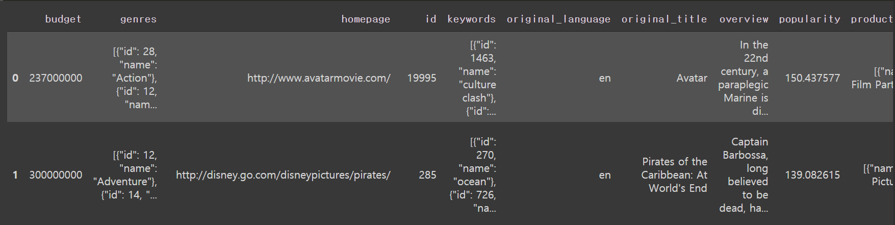

 

 

movies.shape
#(4803,20)

import json

#json에 들어가있는 장르 이름만 빼서 하나의 string으로 만들 것
def add_genre_name(j):
    genres = []
    ar = json.loads(j)
    for a in ar:
        genres.append(a.get("name"))
    return " ".join(sorted(genres))

movies['genres_name'] = movies.apply(lambda x: add_genre_name(x.genres), axis=1)

movies[['genres_name']].head()   # vs. movies['genres_name'].head()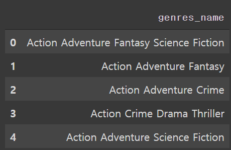

#장르의 unique한 조합
movies['genres_name'].nunique()
#638

#장르의 unique한 조합에 속하는 영화의 갯수
movies.groupby('genres_name').size()

credits.head()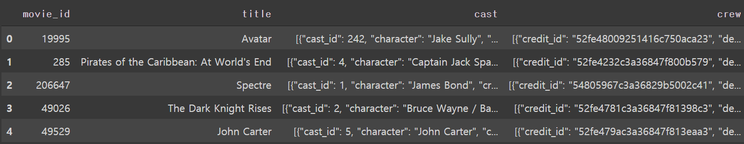

credits.shape
#(4803,4)

2. movies와 credits 데이터 프레임을 조인

#movies의 id와 credits의 movie_id를 이용
movie_credits = pd.merge(movies, credits, left_on='id', right_on='movie_id')
movie_credits.head()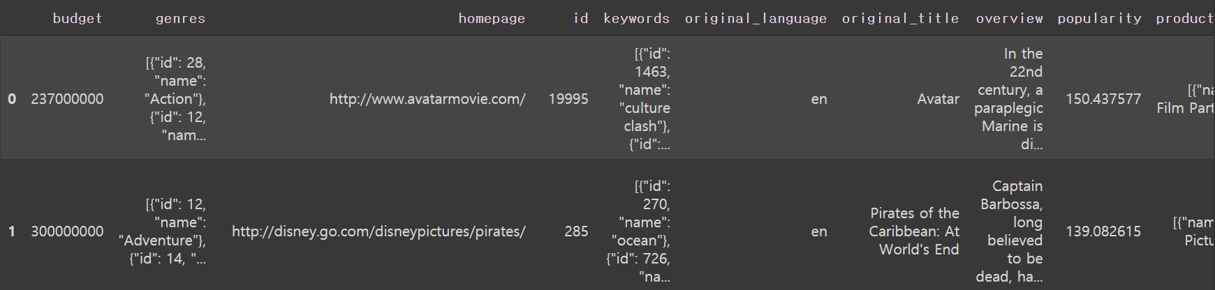

#필요없는 column들 삭제
movie_credits = movie_credits.drop(columns=['homepage', 'title_x', 'title_y', 'status','production_countries', 'production_companies'])
movie_credits.head()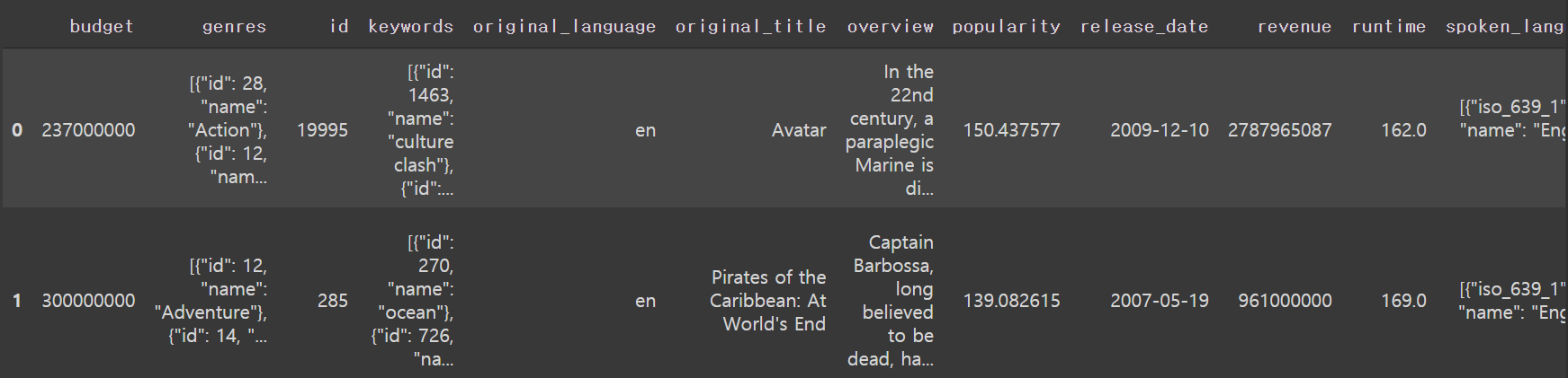

movie_credits.info()
#info()를 통해 비어있는 레코드가 있는 지 확인
#overview, release_date, runtime, tagline에 존재하는 걸 알 수 있음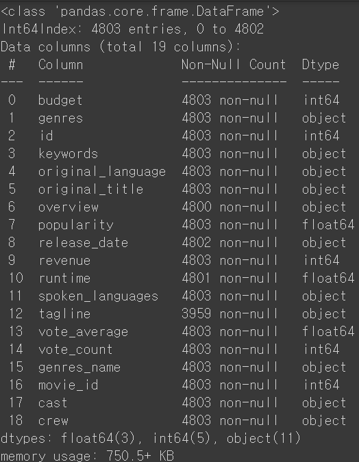

#통계정보출력
movie_credits.describe()

#인기도순으로 내림차순 정렬
popularity = movie_credits.sort_values('popularity',ascending=False)

import matplotlib.pyplot as plt
import seaborn as sns

plt.figure(figsize=(12,6))
ax=sns.barplot(
    x=popularity['popularity'].head(10),
    y=popularity['original_title'].head(10)
)

plt.title('Most Popular by Popularity', weight='bold')
plt.xlabel('Score of Popularity', weight='bold')
plt.ylabel('Movie Title', weight='bold')
plt.savefig('best_popular_movies.png')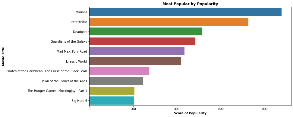

#n개의 인기영화 return(장르는 옵션)
def reco_top_scored_one(n, genre=None):
  if genre is None:
    return popularity["original_title"].head(n)
  else:
    return popularity[popularity['genres_name'].str.contains(genre)]["original_title"].head(n)

#장르값 None으로 인기영화 top 10
print(reco_top_scored_one(10))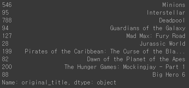

#Science Fiction 장르 중에서 인기영화 top10
print(reco_top_scored_one(10, "Science Fiction"))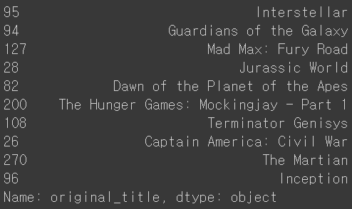

#Action장르 중에서 인기영화 top10
print(reco_top_scored_one(10, "Action"))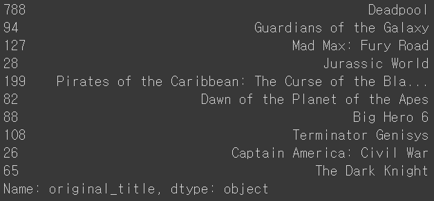

2. 유사도 측정

협업 필터링에서도 유사도 측정은 중요했지만 사용자와 아이템을 '평점'을 기준으로 유사도 측정했었음

컨텐츠 기반 추천에선 아이템이 무엇인지가 중요

ex)옷의 모양, 영화 타이틀, 장르, 배우 정보등을 찾아서 유사한 아이템 추천

이런 방식의 장점 : 부가적인 정보(평점, 리뷰)같은 게 필요가 없음

단점 : 개인화X

다양한 유사도 측정 알고리즘

벡터들간의 유사도를 판단하는 방법

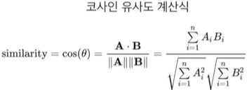
코사인 유사도

n차원 공간에 있는 두 개의 벡터간의 각도르 ㄹ보고 유사도를 판단하는 기준

각도가 비슷한 방향이면 유사도가 높음->코사인값이 1에 가까워짐

각도가 반대 방향이면 유사도가 낮음->코사인값이 -1에 가까워짐

피어슨 유사도

=중앙 코사인 유사도, 보정된 코사인 유사도

코사인 유사도의 개선 버전

방향뿐만 아니라 벡터 크기의 정규화가 중요하면 사용

계산 방법?

1. 벡터 A와 B의 값들을 보정
   • 각 벡터 내 셀들의 평균값을 구한 뒤 평균값을 각 셀에서 빼줌->원점이 중심으로 이동하게 됨
2. 이후 계산은 코사인 유사도와 동일

장점 : 모든 벡터가 원점을 중심으로 이동되기 때문에 벡터간 비교가 쉬워짐

->평점이란 관점에서는 까다로운 사용자와 아닌 사용자를 정규화하는 효과!

3. TF-IDF 소개와 실습

컨텐츠 기반 추천 엔진을 만들려면 텍스트를 행렬(벡터)로 표현하는 방법을 알아야함

1. 원핫인코딩+Bag of Words(카운트)

단어의 수를 카운트해서 표현

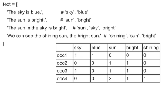
원핫인코딩+Bag of Words(카운트) 예제(수기)

문서에 나오는 단어들을 카운트해서 벡터화시키고 문서 벡터들 간 내적을 하면 유사도 측정!

예제에서 doc1과 doc2는 0이 나오므로 유사도 0, doc1과 doc4도 마찬가지

from sklearn.feature_extracion.text import CountVectorizer
text=[
	'The sky is blue',
    'The sun is bright',
    'The sun in the sky is bright',
    'We can see the shining sun, the bright sun'
    ]
#analyzer='word' : 입력되는 텍스트를 word단위로 끊기
#stop_words='english' : 자주 나오고 의미가 없는 단어들은 무시 ex)if, is, a 등
countvectorizer=CountVectorizer(analyzer='word', stop_words='english')
count_wm=countvectorizer.fit_transform(text)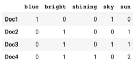

원핫인코딩+Bag of Words(카운트)예제(코드)

2. 원핫인코딩+Bag of Words(TF-IDF)

앞의 카운트 방식은 자주 나오는 단어가 높은 가중치를 갖게됨

한 문서에서 중요한 단어를 카운트가 아닌 문서군 전체를 보고 판단

->어떤 단어가 한 문서에서 자주 나오면 중요하지만 다른 문서들에서는 자주 나오지 않는다면 더 중요!

단어의 값을 TF-IDF 알고리즘으로 계산된 값으로 표현

단순 카운트가 아닌 텍스트가 문서에서 중요한 정도를 측정

 

단어 t의 문서 d에서의 점수 : TF-IDF = TF(t,d)*IDF(t)

• TF(t,d) : 단어 t가 문서 d에서 몇번 나왔는지?
• DF(t) : 단어 t가 전체 문서군에서 몇번 나왔는지?
• IDF(t) : 앞서 DF(t)의 Inverse

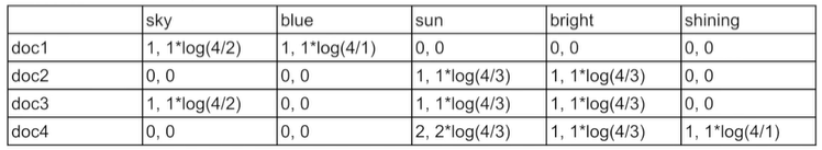
원핫인코딩+Bag of Words(TF-IDF)예제(수기)

ex)'sun'의 doc4에서 TF-IDF점수?

N=4, 'sun'이 나온 문서의 수=3, doc4에서 'sun'의 카운트=2

TF-IDF=2*ln(4/3)=0.575

#tf-idf로 문서 벡터 생성
from sklearn.feature_extraction.text import TfidVectorizer
text=[
	'The sky is blue',
    'The sun is bright',
    'The sun in the sky is bright',
    'We can see the shining sun, the bright sun'
    ]
#여기선 normalization해줌 L2 norm으로 해서 벡터를 단위 벡터(길이가 1인 벡터)로 만듦
tfidfvectorizer=TfidfVectorizer(analyzer='word', stop_words='english', norm='l2')
tfidf_wm=tfidfvectorizer.fit_transform(text)
#scikit-learn의 TF-IDF공식은 ln(N+1)/(DF+1)+1로 조금 다름
#why?ln 1은 0이라 0으로 나누면 에러가 뜨기 때문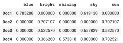

원핫인코딩+Bag of Words(TF-IDF)예제(코드)

#문서 벡터간의 유사도 측정
from sklearn.metrics.pairwise import cosine_similarity

cosine_similarities=cosine_similarity(tfidf_wm)
print(cosine_similarities)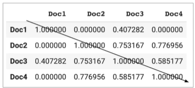

원핫인코딩+Bag of Words(TF-IDF)예제(코드)

->열 또는 행을 기준으로 내림차순으로 정렬하면 해당 문서와 비슷한 문서를 찾을 수 있음

TF-IDF 문제점

• 정확하게 동일한 단어가 나와야 유사도 계산이 이뤄짐(동의어 처리X)
• 단어의 수,아이템 수가 늘어나면 계산이 오래 걸림

->워드 임베딩을 사용하거나 LSA(Latent Semantic Analysis)와 같은 차원 축소 방식 사용

 

실습

1. 카운트 방식의 유사도 계산

from sklearn.feature_extraction.text import TfidfVectorizer, CountVectorizer
import pandas as pd

text = [
   'The sky is blue.',             # ‘sky’, ‘blue’       
   'The sun is bright.',          # ‘sun’, ‘bright’     
   'The sun in the sky is bright',    # ‘sun’, ‘sky’, ‘bright’
   'We can see the shining sun, the bright sun.'  # ‘ see’, ‘shining’, ‘sun’, ‘bright’ 
]


countvectorizer = CountVectorizer(analyzer='word', stop_words='english')
count_wm = countvectorizer.fit_transform(text)
print(count_wm.shape)
print(count_wm.todense())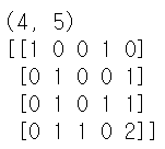

count_tokens = countvectorizer.get_feature_names()
print(count_tokens)
df_countvect = pd.DataFrame(data = count_wm.toarray(), index = ['Doc1','Doc2', 'Doc3', 'Doc4'], columns = count_tokens)
df_countvect.head()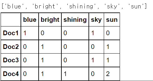

from sklearn.metrics.pairwise import cosine_similarity

cosine_similarities = cosine_similarity(count_wm)
print(cosine_similarities)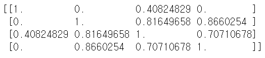

pd.DataFrame(data = cosine_similarities, index = ['Doc1','Doc2', 'Doc3', 'Doc4'], columns = ['Doc1','Doc2', 'Doc3', 'Doc4'])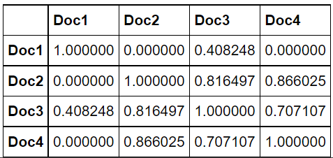

2. TF-IDF방식의 유사도 계산

tfidfvectorizer = TfidfVectorizer(analyzer='word', stop_words='english')

tfidf_wm = tfidfvectorizer.fit_transform(text)
print(tfidf_wm.shape)
print(tfidf_wm.todense())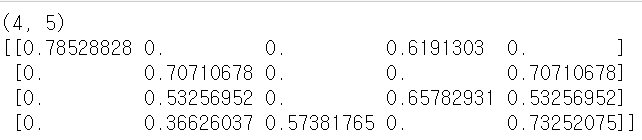

tfidf_tokens = tfidfvectorizer.get_feature_names()
print(tfidf_tokens)
df_tfidfvect = pd.DataFrame(data = tfidf_wm.toarray(), index = ['Doc1','Doc2', 'Doc3', 'Doc4'], columns = tfidf_tokens)
df_tfidfvect.head()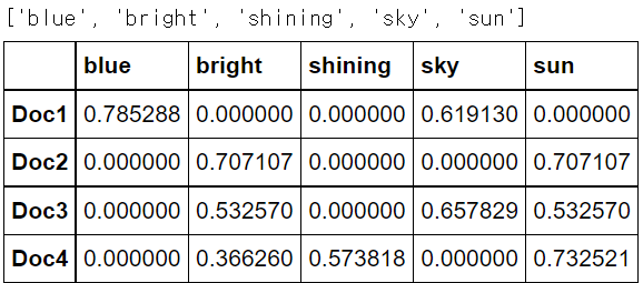

from sklearn.metrics.pairwise import cosine_similarity

cosine_similarities = cosine_similarity(tfidf_wm)
print(cosine_similarities)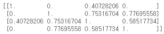

pd.DataFrame(data = cosine_similarities, index = ['Doc1','Doc2', 'Doc3', 'Doc4'], columns = ['Doc1','Doc2', 'Doc3', 'Doc4'])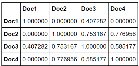

4. TF-IDF를 이용한 컨텐츠 기반 추천 엔진 실습

1. 입력데이터 로딩

영화 정보는 tmdb_5000_movies.csv라는 파일에 존재

import pandas as pd
import numpy as np

movies = pd.read_csv("https://grepp-reco-test.s3.ap-northeast-2.amazonaws.com/tmdb_5000_movies.csv")
movies.head()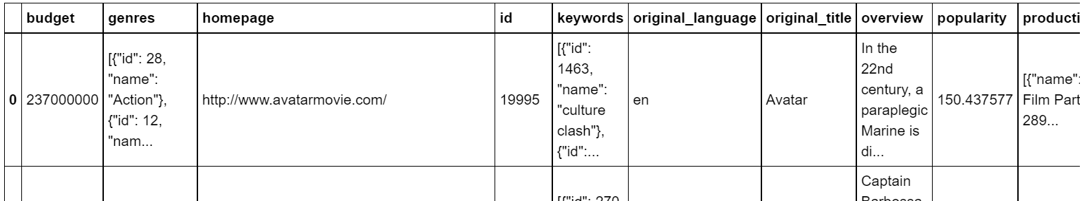

movies.shape
#(4803, 20)

import json

def f(j):
    genres = []
    ar = json.loads(j)
    for a in ar:
        genres.append(a.get("name"))
    return " ".join(sorted(genres))

movies['genres_name'] = movies.apply(lambda x: f(x.genres), axis=1)

movies[['genres_name']].head()   # vs. movies['genres_name'].head()

movies['genres_name'].nunique()
#638

movies.groupby('genres_name').size()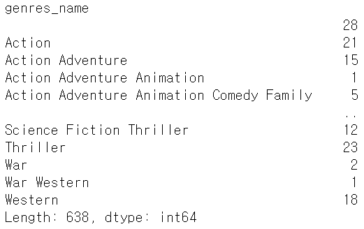

2. 여러 텍스트 필드들을 모아서 텍스트 유사도에 사용할 텍스트 필드 하나를 생성

for f in ['original_title','overview','genres_name']:
  movies[f] = movies[f].fillna('')
  
def combine_features(row):
	try:
		return row['original_title']+" "+row['overview']+" "+row["genres_name"]
	except:
		print ("Error:", row)

movies["combined_features"] = movies.apply(combine_features,axis=1)
movies = movies.reset_index()
movies["combined_features"].head()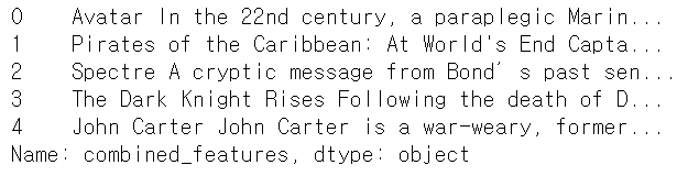

3. TF-IDF 기반 벡터 생성 후 코사인 유사도로 영화들간의 유사도 계산

from sklearn.feature_extraction.text import TfidfVectorizer
from sklearn.metrics.pairwise import cosine_similarity

tfidfvectorizer = TfidfVectorizer(analyzer='word', stop_words='english', norm='l2')
tfidf_matrix = tfidfvectorizer.fit_transform(movies["combined_features"])
tfidf_matrix.shape    #  min_df 파라미터!!!
#(4803, 22179)

cosine_sim = cosine_similarity(tfidf_matrix) # linear_kernel을 사용해도 동일함. tfidf 벡터가 생성될 때 L2 normalization이 되었기 때문
df_cosine_sim = pd.DataFrame(data = cosine_sim)
df_cosine_sim.head()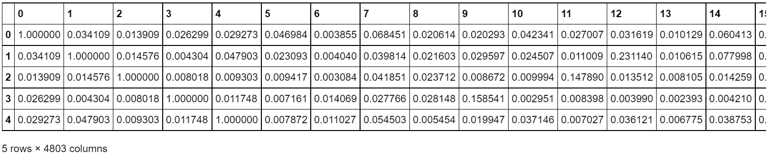

4. 컨텐츠 기반 추천 함수 만들기

def get_title_from_index(df, index):
	return df[df.index == index]["original_title"].values[0]

def get_index_from_title(df, title):
	return df[df.original_title == title]["index"].values[0]
    
cosine_sim[0]
#array([1.        , 0.03410854, 0.01390903, ..., 0.        , 0.        ,0.        ])

for cs in enumerate(cosine_sim[0]):
  print(cs)

def reco_top_similar_movies(movie_title, n=10):
  movie_index = get_index_from_title(movies, movie_title)
  similar_movies =  enumerate(cosine_sim[movie_index])
  sorted_similar_movies = sorted(similar_movies, key=lambda x:x[1], reverse=True)

  ret_movies = []
  i = 0
  for element in sorted_similar_movies:
    title = get_title_from_index(movies, element[0])
    ret_movies.append(title)
    i=i+1
    if i >= n:
      break
  return ret_movies
  
print(reco_top_similar_movies('Avatar', 5))
#['Avatar', 'Apollo 18', 'The American', 'Obitaemyy Ostrov', 'The Matrix']

print(reco_top_similar_movies('Minions', 5))
#['Minions', 'Despicable Me 2', 'Stuart Little 2', 'Stuart Little', 'Austin Powers: The Spy Who Shagged Me']

print(reco_top_similar_movies('Harry Potter and the Half-Blood Prince', 5))
#['Harry Potter and the Half-Blood Prince', 'Harry Potter and the Goblet of Fire', 'Harry Potter and the Order of the Phoenix', 'Harry Potter and the Chamber of Secrets', 'Harry Potter and the Prisoner of Azkaban']